Monte Carlo — stress-test your strategy across 1,000 futures
What the simulation does, exactly how it computes, and how to read the dispersion chart, the percentile table and Kelly.
Backtesting → Monte-Carlo answers the question your backtest cannot: “was my result skill, or one lucky shuffle?” A backtest is a single sample — one specific ordering of wins and losses. Monte Carlo takes the odds behind that sample and replays them across a thousand independent futures, so you see the full range of outcomes your strategy can produce — including the ugly ones.
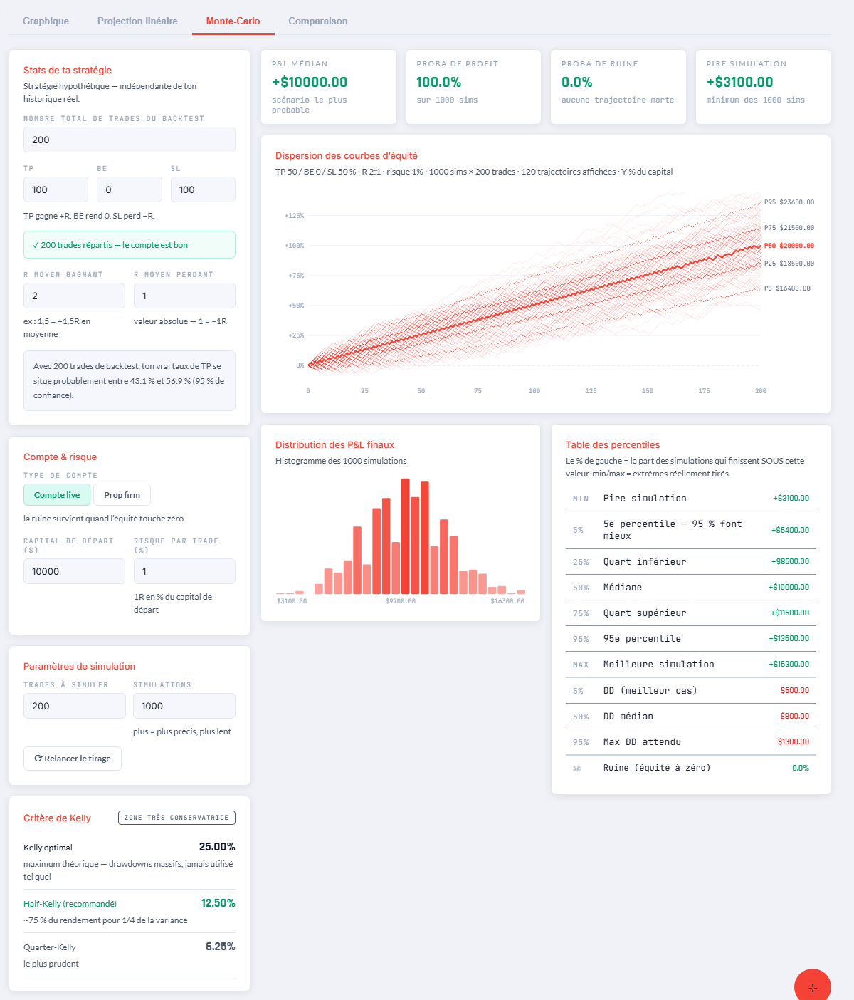
1 · Describe your strategy — in trade counts, not feelings
- Total backtest trades — the size of your sample.
- TP / BE / SL — how many of those trades hit take-profit, broke even, or stopped out. The three must add up to the total: a live checker turns green when the split is exact.
- Average winning R / losing R — what a winner pays and a loser costs, in risk units. 2 and 1 means winners average +2R, losers −1R.
Below the fields, Axel shows a 95% confidence interval on your TP rate: with 200 trades and a 50% hit rate, your true rate probably sits between 43% and 57%. The smaller your sample, the wider that band — and the less your backtest proves.
2 · Account & risk — where ruin gets real
- Live account — a path is ruined when its equity touches zero.
- Prop firm — enter the firm's max allowed drawdown (e.g. 10%): a path is breached the moment equity touches that floor.
3 · What the simulator actually computes
The stake is fixed in dollars: 1R = your risk % × the starting capital (no compounding — position size does not grow with the balance). Then each simulated trade is one random draw with your exact odds:
| Outcome | Probability | Equity moves by |
|---|---|---|
| Take-profit | TP ÷ total | + winning R × stake |
| Break-even | BE ÷ total | 0 |
| Stop-loss | SL ÷ total | − losing R × stake |
One path = that draw repeated over the number of future trades you chose. One simulation run = up to 5,000 such paths. Everything on screen — median, percentiles, drawdowns, ruin — is simply read off those paths. Results recompute live as you type; ⟳ Re-run the draw rolls a fresh set of random futures with the same parameters.
4 · Reading the dispersion chart
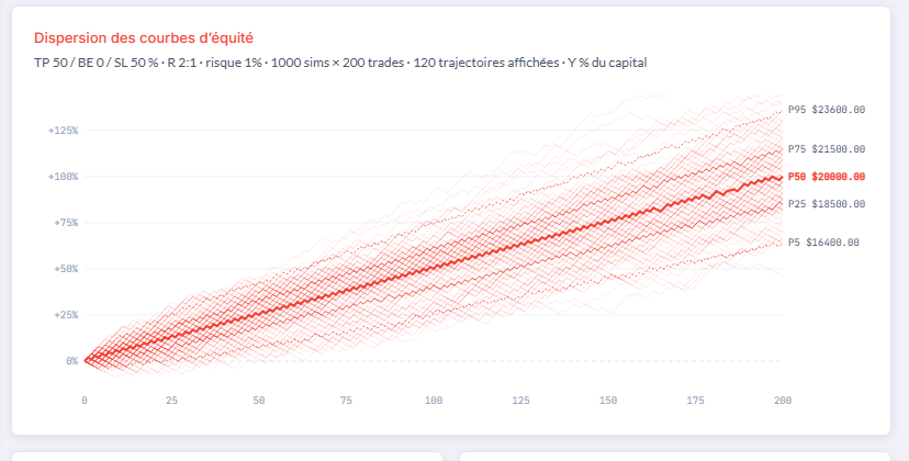
120 of the simulated futures (thin fan), with the percentile bands computed across all of them.
- The fan — each faint line is one complete simulated future, plotted in % of starting capital.
- P50 (bold) — the median: at every trade number, half the futures sit above this line, half below.
- P25 / P75 — the middle half of outcomes lives between these two.
- P5 / P95 (dotted) — the tails: only 1 future in 20 ends below P5, or above P95.
- Red dashed line — the ruin floor (zero, or the prop drawdown limit). Paths that touch it flatline there.
The subtitle above the chart always shows the effective parameters the run used — so an empty or out-of-range field can never change the results silently.
5 · The histogram and the percentile table
The histogram is the same information collapsed to the finish line: the distribution of final P&L across all simulations.
In the percentile table, the left-hand % reads as: “that share of simulations finished below this value.” Two extra rows show the actual worst and best simulations drawn — the true extremes, not percentiles. Note that with a strong edge and reasonable risk, even the worst simulation can finish green: that is not a bug, it is what a real edge looks like across 1,000 futures. Push the risk up and watch the ☠ row instead.
6 · Kelly — how much your edge can carry
The Kelly criterion estimates the risk per trade that maximises long-run growth: f* = p − (1 − p) ÷ b, where p is your win probability among decided trades (break-evens don't count) and b your win/loss R ratio. Full Kelly is a theoretical ceiling with brutal drawdowns — that's why the card highlights Half-Kelly and shows a badge placing your risk input relative to those levels.
7 · Honest limits
- Fixed stake — no compounding. It keeps runs comparable; your real curve will differ if you scale size with balance.
- Independent trades — the model assumes every trade has the same odds, independent of the previous one. No regime changes, no tilt, no news days.
- Garbage in, garbage out — the simulation is exactly as good as the backtest numbers you feed it. That's what the sample-size confidence interval is there to remind you.
Monte Carlo doesn't predict your future — it shows the range of futures your current edge makes possible. If the 5th percentile of that range still fits your risk tolerance, you're sizing correctly.